Julia Word Embedding Layer in Flux - Pre-trained GloVe

This example follows on from tutorial #1 in which we trained our own embedding layer. This time we use pre-trained word vectors (GloVe) instead of learning them. We’ll skip over some of the explanations as this is covered in tutorial #1.

As before, the objective for this exercise is to machine learn the sentiment of 10 string arrays. The idea came from this tutorial written by Jason Brownlee who used Keras on a similar dataset.

using  Languages, TextAnalysis, Flux, PyPlot, Statistics

#Display Flux Version
import Pkg ; Pkg.installed()["Flux"]

v"0.7.2"

Data Preparation

This code block is the same as tutorial #1. See this for more explanation.

Arr = ["well done",
     "good work",
     "great effort",
     "nice work",
     "excellent",
     "weak",
     "poor effort",
     "not good",
     "poor work",
     "could have done better"]

# positve or negative sentiment to each 'document' string
y = [true true true true true false false false false false]

docs=[]
for i in 1:length(Arr)
    push!(docs, StringDocument(Arr[i]))
end
crps=Corpus(docs)    
update_lexicon!(crps)
doc_term_matrix=DocumentTermMatrix(crps)
word_dict=doc_term_matrix.column_indices

tk_idx(s) = haskey(word_dict, s) ? i=word_dict[s] : i=0

function pad_corpus(c, pad_size)
    M=[]
    for doc in 1:length(c)
        tks = tokens(c[doc])
        if length(tks)>=pad_size
            tk_indexes=[tk_idx(w) for w in tks[1:pad_size]]
        end
        if length(tks)<pad_size
            tk_indexes=zeros(Int64,pad_size-length(tks))
            tk_indexes=vcat(tk_indexes, [tk_idx(w) for w in tks])
        end
        doc==1 ? M=tk_indexes' : M=vcat(M, tk_indexes')
    end
    return M
end

pad_size=4
padded_docs = pad_corpus(crps, pad_size)
x = padded_docs'
data = [(x, y)]

Flux Embedding Preparation

Load the pre-trained embeddings

This function loads the pre-trained GloVe embeddings. Try Embeddings.jl for a better way to do this if you can get it to work.

function load_embeddings(embedding_file)
    local LL, indexed_words, index
    indexed_words = Vector{String}()
    LL = Vector{Vector{Float32}}()
    open(embedding_file) do f
        index = 1
        for line in eachline(f)
            xs = split(line)
            word = xs[1]
            push!(indexed_words, word)
            push!(LL, parse.(Float32, xs[2:end]))
            index += 1
        end
    end
    return reduce(hcat, LL), indexed_words
end

We’ll use one of the smaller embedding files (glove.6B.50d.txt) as this problem is trivial. This file can be downloaded from here and must reside in the current working folder.

embeddings, vocab = load_embeddings("glove.6B.50d.txt")
embed_size, max_features = size(embeddings)
println("Loaded embeddings, each word is represented by a vector with $embed_size features. The vocab size is $max_features")

Loaded embeddings, each word is represented by a vector with 50 features. The vocab size is 400000

This function provides the index of a word in the GloVe embedding.

#Function to return the index of the word in the embedding (returns 0 if the word is not found)
function vec_idx(s)
    i=findfirst(x -> x==s, vocab)
    i==nothing ? i=0 : i 
end

This function provides the GloVe word vector of the given word.

wvec(s) = embeddings[:, vec_idx(s)]
wvec("done")

Here you can see the GloVe vector representation of one of our words “done”.

50-element Array{Float32,1}:
  0.33076  
 -0.4387   
 -0.32163  
 -0.4931   
  0.10254  
 -0.0027421
 -0.5172   
  0.024336 
 -0.12816  
  0.14349  
 -0.16691  
  0.56121  
 -0.56241  
  ⋮        
  0.060552 
 -0.16143  
 -0.26668  
 -0.1766   
  0.01582  
  0.25528  
 -0.096739 
 -0.097282 
 -0.084483 
  0.33312  
 -0.22252  
  0.74457  

Embedding Preparation

N = size(padded_docs,1)  #Number of documents (10)
max_features = 50
vocab_size = 20

The next block of code initializes a random embedding matrix as per the size of our vocab.

embedding_matrix=Flux.glorot_normal(max_features, vocab_size)

Now we overwrite the random embedding matrix with our word vectors from GloVe. The word vectors are inserted as columns as per the index from word_dict plus 1. The reason we add 1 is so that 0 can represent a zero-word that has been padded.

for term in doc_term_matrix.terms
    if vec_idx(term)!=0
        embedding_matrix[:,word_dict[term]+1]=wvec(term)
    end
end   

Buliding the Model and Training

m = Chain(x -> embedding_matrix * Flux.onehotbatch(reshape(x, pad_size*N), 0:vocab_size-1),
          x -> reshape(x, max_features, pad_size, N),
          x -> sum(x, dims=2),
          x -> reshape(x, max_features, N),
          Dense(max_features, 1, σ)
)

The model (m) needs some explanation.

Layer 1. The first layer’s embedding function matches the words in each document to corresponding word vectors. This is done by rolling all the word vectors one after the other and using onehotbatch to filter out the unwanted words. The output is a 50x40 array.

Layer 2. Unrolls the vectors into the shape 50x4x10; i.e. 8 features and 10 documents of padded size 4.

Layer 3. Now that our data is in the shape provided by layer 2 we can sum the word vectors to get an overall ‘meaning’ vector for each document. The output is now in the shape size of 50 x 1 x 10.

Layer 4: Drops the axis (1) so that the shape of x is a size suitable for training. After this step the shape is 50x10.

Layer 5: is a normal Dense layer with the sigmoid activation function to give us nice probabilities.

If you’d like to see each layer in action I recommend usingm[1](x) to see sample output from the first layer. m[1:2](x) to see output from the second layer and so on.

loss_h=[]
accuracy_train=[]
accuracy(x, y) = mean(x .== y)

As this is a binary (1 or 0) classification problem we need to use binarycrossentropy to calculate the loss. The optimizer is gradient descent.

loss(x, y) = sum(Flux.binarycrossentropy.(m(x), y))
optimizer = Flux.Descent(0.001)

Train the model

for epoch in 1:400
    Flux.train!(loss, Flux.params(m), data, optimizer)
    #println(loss(x, y).data, " ", accuracy(m(x).>0.5,y))
    push!(loss_h, loss(x, y).data)
    push!(accuracy_train, accuracy(m(x).>0.5,y))
end
println(m(x).>0.5)
accuracy(m(x).>0.5,y)

Bool[true true true true true false false false false false]
1.0

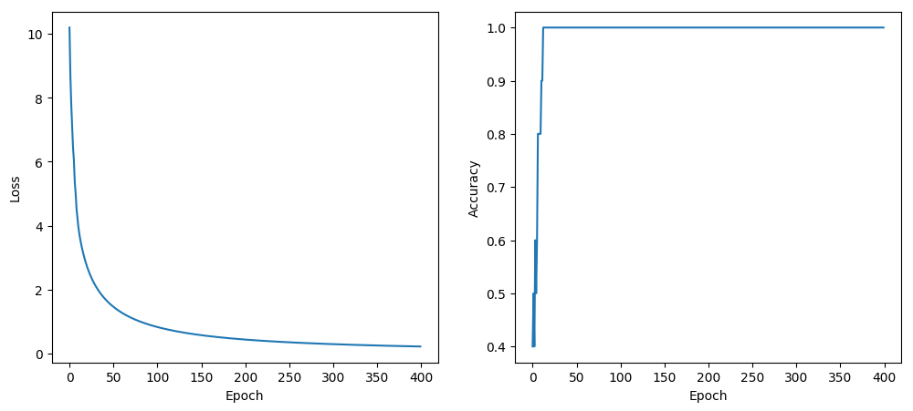
Outputs over 0.5 are considered positive (true) and our final accuracy this time is 100%.

figure(figsize=(12,5))

subplot(121)
PyPlot.xlabel("Epoch")
ylabel("Loss")
plot(loss_h)

subplot(122)
PyPlot.xlabel("Epoch")
ylabel("Accuracy")
plot(accuracy_train, label="train")

Note, I think some parts of this could be done more elegantly, let me know if anything could be improved (I’m still learning too).