Julia Project - Monte Carlo Simulation for Investment Portfolio Earnings

Introduction

In this notebook we use Julia to look at typical investment risk profiles and employ the Monte Carlo method with Geometric Brownian motion (GBM) to simulate the growth of an investment portfolio.

The simulations do not take into account any ongoing payments or tax. Nor do they encompass other factors such as inflation.

Note, do not rely on any part of this article for your own personal circumstances. This is not financial advice!

With the disclaimer out of the way let’s begin as usual by loading the Julia libraries we’ll need.

using DataFrames, CSV, Distributions, PyPlot, Dates, Statistics, StatsFuns

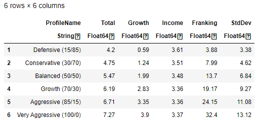
Now let’s load in our risk profile data. Users of the financial software XPLAN will recognise headings used in this dataframe. We only actually need the data from the ‘Total’ column being the overall expected growth (Growth + Income) and ‘StdDev’ which is the risk profile’s standard deviation.

df=CSV.read("/mnt/juliabox/Monte Carlo/assumptions.csv")

What is a Risk Profile

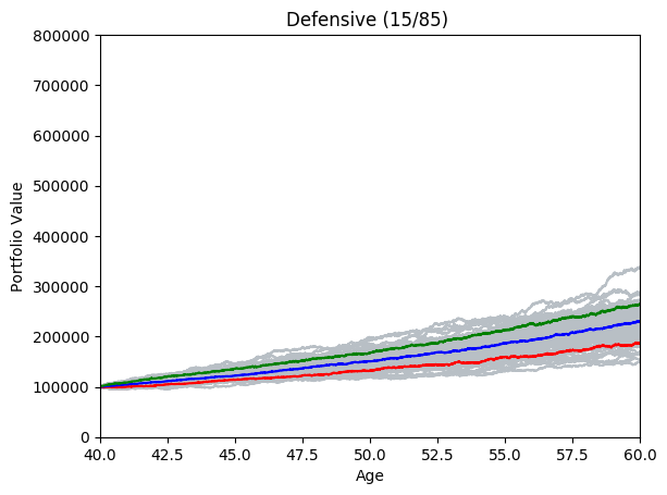
A risk profile is an evaluation of an individual’s willingness and ability to take risks. Financial Advisers often fit client’s into one of several risk profiles after asking them discovery questions. The risk profile names and values above have been made up but they are indicative of real values. The first risk profile ‘Defensive’ is made up from 15% growth assets and 85% defensive assets; this risk profile would suit a cautious investor who wants to make steady progress without taking too much risk. At the other end of the table a ‘Very Aggressive’ risk profile is made up from 100% growth assets and would suit an individual who is more willing to take a risk to gain higher returns.

The function below plots a normal distribution curve of a given risk profile.

function plot_rp(rp)
    μ = df[rp,:].Total
    σ = df[rp,:].StdDev
    dist = Normal(μ, σ)
    x = μ - 3σ : 0.01 : μ + 3σ
    plot(x, pdf(dist,x), label=df[rp,:].ProfileName)
    legend(loc="upper right", fontsize = "small")
    axis([-30,50,0,0.12])
    title("Normal Distribution")
    axvline(x=0, color="k", linestyle="--")
    xlabel("Annual Growth (%)")
    ylabel("PDF")
end

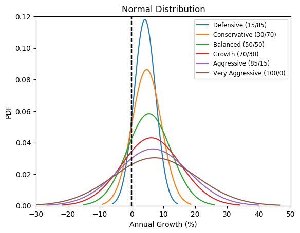
Let’s plot all the curves and then interpret the output.

for rp in 1:length(df)
    plot_rp(rp)
end

Interpretation

• The vertical dotted line shows the boundary of positive growth (i.e. making money) vs negative growth (i.e. losing money).

• The first and least risky investment profile is ‘Defensive’. You can observe that probability of achieving the mean total growth of 4.2% is the highest and most of the bell curve area is in the positive growth area.

• The last and most risky investment profile is ’Very Aggressive’. You can observe that the probability of achieving the mean total growth of 7.27% is the lowest. The elongated bell curve shape means there is scope to earn much higher returns at the expense of possible negative returns.

For more information on Probability Distributions click here

Deterministic Prediction Function

The following function makes a deterministic prediction of the future portfolio value based on the following parameters: -

P is the original principal sum

r is the nominal annual interest rate

n is the compounding frequency

t is the overall length of time the interest is applied (expressed using the same time units as r, usually years).

This prediction assumes no additional contributions and perfect market conditions. For more information see this article on Periodic Compounding.

deterministic_predict(P, r , n, t) = P*(1 + r/n)^(n*t)

#Example 1 from wikipedia as a first sanity check
#Suppose a principal amount of $1,500 is deposited in a bank paying an annual interest rate of 4.3%, compounded quarterly.
#Then the balance after 6 years is found by using the formula above, with P = 1500, r = 0.043 (4.3%), n = 4, and t = 6:

deterministic_predict(1500.0 , 0.043, 4.0, 6.0)

1938.8368221341054

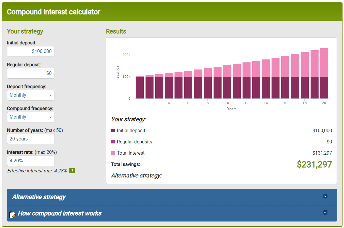
Now let’s apply this function to a retirement saving scenario. Our client is age 40 and wants to retire in 20 years’ time. They currently have $100,000 in their retirement portfolio. What will their balance be like at age 60?

First let’s set a couple of variables and functions that will come in useful.

original_principle_sum=100000 #          Initial portfolio value
interest_rate(rp) = df[rp,:].Total/100 # Simple function to get a risk profile's growth interest rate

Here’s another test output of the function for risk profile 1 (Defensive). For this test let’s assume the interest compounds monthly (12 times a year for each of the 20 years).

deterministic_predict(original_principle_sum, interest_rate(1), 12, 20)

231297.23315323537

By using the Moneysmart Compound Interest Calculator as a second sanity check we can see our deterministic function is working.

Stochastic Prediction Function

The reality with real share portfolios is that unit prices fluctuate up and down on a daily basis. Price fluctuations are generally more volatile for stocks that have the potential to earn more income for the investor. The function below uses Geometric Brownian motion (GBM) to simulate randomised returns based on the given risk profiles. Additional parameters are built into the function to repeat the GBM simulations over-and-over to generate what is known as a Monte Carlo experiment.

Here are some animated gifs showing 20 simulations per risk profile.

The animated gifs below show 20 simulations per risk profile. We can see that as we take more risk the simulations become more volatile.

These gifs were generated with the functions below. Let’s take a closer look at the code used. we start by setting up the known variables and add a few useful functions at the same time.

age=40 #                                 Age at start of projections
frequency = 252 #                        Assume 252 trading days per year
days = 1/frequency #                     Convenient way to express days
yrs_to_days(x)=x*frequency #             Simple function to convert years to days
sigma(rp) = df[rp,:].StdDev/100 #        Simple function to get a risk profile's standard deviation

Now we build the Monte Carlo function. Calling the function produces a matplotlib (PyPlot) chart based on the input parameters. I’ve included some comments in the code but if you need to more depth insight I recommend this great video which gave me the math needed.

function montecarlo(rp, N, iterations, show_Q)
    # rp = the index of the risk profile to use
    # N = Number of years forward to project
    # iterations - no of times to iterate and produce a simulation
    # show_Q - if True, so quantile lines
    
    growth = interest_rate(rp)
    
    # Periodic Daily Return (PDR)
    pdr = log(deterministic_predict(1, growth, frequency, 2*days) / deterministic_predict(1, growth, frequency, 1*days))
    pdr_std = sigma(rp) * sqrt(days)
    pdr_var = pdr_std^2
    drift = pdr - (pdr_var/2)
    
    predictions_all=[]
    
    axis([40,60,0,800000])
    title(df[rp,:].ProfileName)
    xlabel("Age")
    ylabel("Portfolio Value")
    
    for s in 1:iterations
        predictions=[]
        global df_pred=DataFrame(Age = Float64[], MC_Price = Float64[],MC_Balance = Float64[], Deterministic_Balance = Float64[])
        last_price = 1
        for i in 0:yrs_to_days(N)
            i==0 ? mc_price=1 : mc_price=last_price*exp(drift+pdr_std*norminvccdf(rand()))
            push!(df_pred, [age+i*days,
                    mc_price,
                    original_principle_sum*mc_price,
                    deterministic_predict(original_principle_sum, growth, frequency, i*days)])
            push!(predictions, original_principle_sum*mc_price)
            last_price = mc_price
        end
        s == 1 ? predictions_all = predictions : predictions_all = hcat(predictions_all, predictions)
        plot(df_pred[:Age], df_pred[:MC_Balance], color="#B8BFC5", label="Monte Carlo Iteration")
    end 
    if show_Q
        #Show quantile predictions
        df_Q = DataFrame(Age = Float64[], Q1 = Float64[], Q5 = Float64[], Q9 = Float64[])
        for i in 1:yrs_to_days(N)
            push!(df_Q, [age+i*days,
                    quantile(predictions_all[i,:],0.1),
                    quantile(predictions_all[i,:],0.5),
                    quantile(predictions_all[i,:],0.9)])
        end
        plot(df_Q[:Age], df_Q[:Q1], color="r", label="10th Percentile")
        plot(df_Q[:Age], df_Q[:Q5], color="b", label="50th Percentile")
        plot(df_Q[:Age], df_Q[:Q9], color="g", label="90th Percentile") 
    else
        plot(df_pred[:Age], df_pred[:Deterministic_Balance], color="b", label="Deterministic Prediction")   
    end
end

The following code was used to produce a sequence of PNG image files that I later used to create the animated gifs above. I used a free app for the Mac called PicGIF lite to generate the final animated gifs.

using PyCall
@pyimport matplotlib.animation as anim

fig = figure(figsize=(5,4))

for rp in 1:length(df)
    withfig(fig) do
        for k in 1:20
            clf()
            montecarlo(rp, 20, 1, false)
            savefig("rp_" * string(rp) *  "_" * string(k), bbox_inches="tight")
        end
    end
end

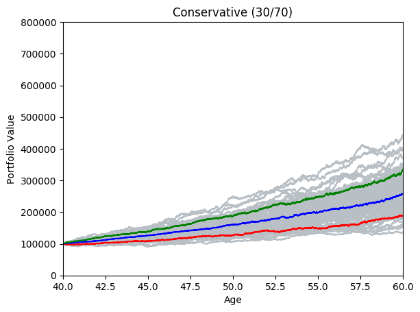
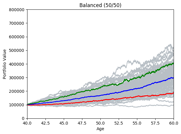
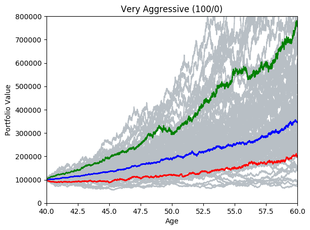
By running many simulations (see grey lines below) we can take the mean and quantiles each of each day’s simulations and after a while we start to see deterministic predictions emerging. The area between green and blue can be interpreted as ‘good’ market conditions. The area between the blue and the red would be ‘bad’ market conditions.

# Terminal command line to zip up the PNG files.
# zip rp.zip rp*

montecarlo(1, 20, 100, true)

montecarlo(2, 20, 100, true)

montecarlo(3, 20, 100, true)

montecarlo(4, 20, 100, true)

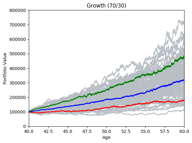
montecarlo(5, 20, 100, true)

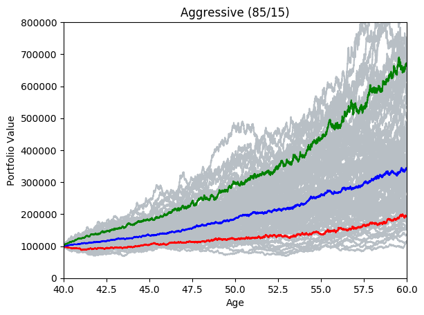
montecarlo(6, 20, 100, true)