

Julia Project - Song Lyric Text Classification by Artist
I had an idea for a work-related project I’d like to do some day given the opportunity. The objective would be to build a machine learning model that can classify notes or documents for compliance purposes. To get such a project off the ground sufficient labelled training data would be needed. There isn’t going to be the luxury of trained data like the famous IMDb data set which contains 50,000 labelled movie reviews. The data we would obtain would likely be less than 1000 rows (at least to start with).
So I went on a search for trained text data sets and somehow ended up with this Song Lyric dataset from Kaggle. I thought it would be a fun challenge to pick 5 popular artists who had made many songs and try to build a model that could predict the artist who sung the song with test data unseen by the training step. The filtered dataset used for training is less than 800 rows making it kind of comparable to the work-related project I had in mind.
The task of predicting the artist isn’t quite as straightforward as you first think; each artist will likely have songs in different genres (e.g. upbeat, downbeat and ballads). The songs may have been written by different band members and will also be of variable length. Just guessing the artist correctly is going to be a 1 in 5 chance or (0.2 probability).
This project brings together all my recent Julia blog post learnings with NLP, Flux, Neural Networks and Convolutional Neural Networks, (i.e. CNN’s or ConvNets). An added challenge was the lack of similar examples on the web for Word Embeddings with Flux or Word Embeddings with Flux CNN’s. I’m quite proud I got these working without having to copy anyone else’s work. The code may not be super-pretty but it works!!
Let’s get started loading the libraries we need.
using CSV, DataFrames, Random, TextAnalysis, Languages, Statistics, PyPlot, Flux, BSON

#Display Flux Version
import Pkg ; Pkg.installed()["Flux"]
loaded
v"0.7.2"
Loading and Initial Data Preparation
Load the data from the CSV file we downloaded from Kaggle and show a count of all songs.
df_all=CSV.read("/mnt/juliabox/NLP/songdata.csv")
categorical!(df_all, :artist)
show(by(df_all, :artist, nrow))
643×2 DataFrame
│ Row │ artist        │ x1    │
├─────┼───────────────┼───────┤
│ 1   │ 'n Sync       │ 93    │
│ 2   │ ABBA          │ 113   │
│ 3   │ Ace Of Base   │ 74    │
│ 4   │ Adam Sandler  │ 70    │
│ 5   │ Adele         │ 54    │
│ 6   │ Aerosmith     │ 171   │
│ 7   │ Air Supply    │ 174   │
⋮
│ 636 │ Zeromancer    │ 30    │
│ 637 │ Ziggy Marley  │ 64    │
│ 638 │ Zoe           │ 1     │
│ 639 │ Zoegirl       │ 38    │
│ 640 │ Zornik        │ 12    │
│ 641 │ Zox           │ 21    │
│ 642 │ Zucchero      │ 30    │
│ 643 │ Zwan          │ 14    │
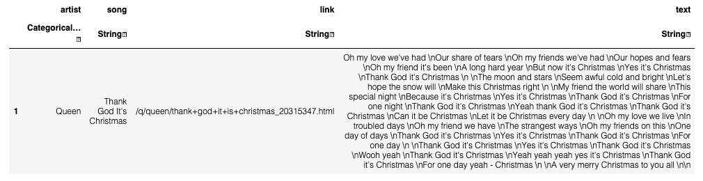
This is a great dataset but we need to make a new dataframe containing just the song lyrics and labelled artists selected. The data is randomly shuffled using a known ‘seed’ so we can replicate the same order each time the notebook is run. The first row of data is output.
artists=["Queen", "The Beatles", "Michael Jackson", "Eminem", "INXS"]
df=df_all[[x in artists for x in df_all[:artist]],:]
df_all=nothing
Random.seed!(1000);
df=df[shuffle(1:size(df, 1)),:]
df[1,:]
size(df,1)
727
This size of the dataset is only 727 rows – a shortage of examples will mean this is likely to be a hard task!
Preprocessing - clean-up
The next block of code uses the TextAnalysis library to create a corpus of our song lyrics and cleans it for the next step.
docs=Any[]
for i in 1:size(df,1)
    txt=df.text
    txt=replace(df[i,:].text, "\n" => " ")
    txt=replace(df[i,:].text, "'" => "")
    dm=TextAnalysis.DocumentMetadata(Languages.English(), df[i,:].song,"","")
    doc=StringDocument(txt, dm)
    push!(docs, doc)
end
crps=Corpus(docs)
orig_corpus=deepcopy(crps);
prepare!(crps, strip_non_letters | strip_punctuation | strip_case | strip_stopwords | strip_whitespace)
Let’s take a look at the first song to see what just took place. In the original corpus the first song by Queen looked like this.
orig_corpus[1]
StringDocument{String}("Oh my love weve had \nOur share of tears \nOh my friends weve had \nOur hopes and fears \nOh my friend its been \nA long hard year \nBut now its Christmas \nYes its Christmas \nThank God its Christmas \n \nThe moon and stars \nSeem awful cold and bright \nLets hope the snow will \nMake this Christmas right \n \nMy friend the world will share \nThis special night \nBecause its Christmas \nYes its Christmas \nThank God its Christmas \nFor one night \nThank God its Christmas \nYeah thank God its Christmas \nThank God its Christmas \nCan it be Christmas \nLet it be Christmas every day \n \nOh my love we live \nIn troubled days \nOh my friend we have \nThe strangest ways \nOh my friends on this \nOne day of days \nThank God its Christmas \nYes its Christmas \nThank God its Christmas \nFor one day \n \nThank God its Christmas \nYes its Christmas \nThank God its Christmas \nWooh yeah \nThank God its Christmas \nYeah yeah yeah yes its Christmas \nThank God its Christmas \nFor one day yeah - Christmas \n \nA very merry Christmas to you all \n\n", TextAnalysis.DocumentMetadata(Languages.English(), "Thank God It's Christmas", "", ""))
After the pre-processing step it looked like this.
crps[1]
StringDocument{String}("oh love weve share tears oh friends weve hopes fears oh friend hard christmas christmas thank god christmas moon stars awful cold bright hope snow christmas friend world share special night christmas christmas thank god christmas night thank god christmas yeah thank god christmas thank god christmas christmas christmas day oh love live troubled days oh friend strangest oh friends day days thank god christmas christmas thank god christmas day thank god christmas christmas thank god christmas wooh yeah thank god christmas yeah yeah yeah christmas thank god christmas day yeah christmas merry christmas ", TextAnalysis.DocumentMetadata(Languages.English(), "Thank God It's Christmas", "", ""))
Preprocesing - prep for training
The update lexicon commands will quickly count our words and consequently let us lookup words to see in which songs they occur.
update_lexicon!(crps)
update_inverse_index!(crps)
The word “christmas” is located in the song corpus with these indexes
crps["christmas"]
8-element Array{Int64,1}:
   1
 162
 239
 328
 332
 490
 606
 638
The following code builds our word dictionary (word_dict).
Each word in our song corpus can now be represented by a unique integer.
m_dtm=DocumentTermMatrix(crps)
word_dict=m_dtm.column_indices
Dict{String,Int64} with 8449 entries:
  "ont"         => 5080
  "youd"        => 8421
  "bsta"        => 897
  "enjoy"       => 2388
  "chocolate"   => 1226
  "fight"       => 2675
  "null"        => 5007
  "princess"    => 5603
  "snuggle"     => 6777
  "carousels"   => 1068
  "needin"      => 4914
  "helping"     => 3378
  "manufacture" => 4437
  "sheezy"      => 6462
  "sleepless"   => 6682
  "favor"       => 2612
  "henry"       => 3391
  "eddie"       => 2303
  "aaaah"       => 5
  "borders"     => 779
  "tenor"       => 7459
  "star"        => 7001
  "prick"       => 5594
  "worship"     => 8340
  "itll"        => 3775
  ⋮             => ⋮
This function returns the word_dict index value of the word passed in s. It returns 0 if the word is not found.
tk_idx(s) = haskey(word_dict, s) ? i=word_dict[s] : i=0
tk_idx (generic function with 1 method)
Let’s try it out.
tk_idx("christmas")
1249
For the training step all the songs need to be the same length of words and the words need converting to numbers. The following function performs this task by padding shorter songs with zeros and truncating longer songs to the size specified.
function pad_corpus(c, size)
    M=[]
    for doc in 1:length(c)
        tks = tokens(c[doc])
        if length(tks)>=size
            tk_indexes=[tk_idx(w) for w in tks[1:size]]
        end
        if length(tks)<size
            tk_indexes=zeros(Int64,size-length(tks))
            tk_indexes=vcat(tk_indexes, [tk_idx(w) for w in tks])
        end
        doc==1 ? M=tk_indexes' : M=vcat(M, tk_indexes')
    end
    return M
end
pad_corpus (generic function with 1 method)
num_terms_in_songs=[length(tokens(crps[i])) for i in 1:length(crps)]
println("min $(minimum(num_terms_in_songs)) max $(maximum(num_terms_in_songs)) mean $(mean(num_terms_in_songs))")
min 19 max 400 mean 99.43053645116919
We can see that the mean is around 100 words, however, I found (when hyperparameter tuning) that a higher number improved accuracy. We will set doc_pad_size to 200.
X becomes our training data which is now in a format suitable for input into a neural network model.
doc_pad_size=200
padded_docs = pad_corpus(crps, doc_pad_size)
X = padded_docs'
200×727 LinearAlgebra.Adjoint{Int64,Array{Int64,2}}:
    0     0     0     0     0     0  …     0     0     0     0     0     0
    0     0     0     0     0     0        0     0     0     0     0     0
    0     0     0     0     0     0        0     0     0     0     0     0
    0     0     0     0     0     0        0     0     0     0     0     0
    0     0     0     0     0     0        0     0     0     0     0     0
    0     0     0     0     0     0  …     0     0     0     0     0     0
    0     0     0     0     0     0        0     0     0     0     0     0
    0     0     0     0     0     0        0     0     0     0     0     0
    ⋮                             ⋮  ⋱                             ⋮
 8398  7460  1684  5002  7490  4321     3472  4321  7863  3667  3456  3269
 8398  3456  5061  1144   409  2632     1180   409  6799  6839  3244  4677
 8398  7580  8423   833  3623  4408  …  7733  3021  3168  3623  3456  4326
 1249  6817  3028   915  1093  4321     2524  4321  1803  3071  3244  1564
 7482  6372  4220  6472  7562  2632     4448   409  5576  3667  3456  4186
 3064  2122  3623  4968  7368  4408     6630  3021  6921  3667  3456  7618
 1249  1684  8309  4968  4189  4321     3676  5083  7589  3623  3456  1684
 1801  8398  3575  8092  3614  2632  …  5448  4321  3177  3071  3456  3699
 8398  8398  8423  4859  2823  4408     3377   409  7631  3667  3456  2182
 1249  8398  7589  7057   582  4321     7652   409  3991  1092  3244  3211
 4579  8398  7589  3956  3338  8398     4562  5083  7636  7490  3456  3754
 1249  8398  7589  1243  2823  2632     7458  3021   622   411  3244  4368
Our data labels y (i.e artists) also need processing into a one-hot-matrix for classification. First let’s define a dictionary of artists called artist_dict.
artist_dict = Dict()
for (n, a) in enumerate(unique(df.artist))
   artist_dict["$a"] = n
end
artist_dict
Dict{Any,Any} with 5 entries:
  "Queen"           => 1
  "Eminem"          => 5
  "The Beatles"     => 3
  "Michael Jackson" => 4
  "INXS"            => 2
We’ll now use onehotbatch magic to make the required transformation for this classification problem.
artist_indexes=[artist_dict[df[:artist][i]] for i in 1:size(df,1)]
y = Flux.onehotbatch(artist_indexes, 1:5)
5×727 Flux.OneHotMatrix{Array{Flux.OneHotVector,1}}:
  true  false  false   true  false  …  false  false  false  false  false
 false   true  false  false  false     false  false  false  false   true
 false  false   true  false  false     false   true  false  false  false
 false  false  false  false   true      true  false   true   true  false
 false  false  false  false  false     false  false  false  false  false
Let’s now split our X data into training and test data sets.
-
Training data will be used to ‘train’ the model.
-
Test data will be new ‘unseen’ data used to make new predictions. As we have knowledge of the artists we will be able to score the accuracy of the model.
X_train = X[:, 1:649]
y_train = y[:,1:649]
X_test = X[:, 650:end]
y_test = y[:, 650:end]

println("X_train $(size(X_train)) y_train $(size(y_train)) X_test $(size(X_test)) y_test $(size(y_test))")
X_train (200, 649) y_train (5, 649) X_test (200, 78) y_test (5, 78)
The final preprocessing step neatly combines our training data and labels into a training_set tuple for Flux.
train_set = [(X_train, y_train)]
1-element Array{Tuple{Array{Int64,2},Flux.OneHotMatrix{Array{Flux.OneHotVector,1}}},1}:
 ([0 0 … 0 0; 0 0 … 0 0; … ; 4579 8398 … 7635 3929; 1249 8398 … 7454 3038], [true false … false false; false true … true false; … ; false false … false false; false false … false true])
Embedding Prep
Our X data is now numbers and these numbers point to words in the word_dict. In it’s current state the numbers don’t really have all that much value for training. The next step is to load the GloVe word embeddings and prepare them as the first layer in our Flux neural network. Word embeddings give our words ‘meaning’ and have been covered in detail in my previous blog posts; please refer to these if you need more background on word vectors and embedding them in Neural Networks.
Let’s load in the embeddings.
function load_embeddings(embedding_file)
    local LL, indexed_words, index
    indexed_words = Vector{String}()
    LL = Vector{Vector{Float32}}()
    open(embedding_file) do f
        index = 1
        for line in eachline(f)
            xs = split(line)
            word = xs[1]
            push!(indexed_words, word)
            push!(LL, parse.(Float32, xs[2:end]))
            index += 1
        end
    end
    return reduce(hcat, LL), indexed_words
end
load_embeddings (generic function with 1 method)
Note we have gone for the 300 dimension file this time for better results.
embeddings, vocab = load_embeddings("glove.6B.300d.txt")
embed_size, max_features = size(embeddings)
println("Loaded embeddings, each word is represented by a vector with $embed_size features. The vocab size is $max_features")
Loaded embeddings, each word is represented by a vector with 300 features. The vocab size is 400000
Now we define our usual functions for returning word vectors.
#Function to return the index of the word 's' in the embedding (returns 0 if the word is not found)
function vec_idx(s)
    i=findfirst(x -> x==s, vocab)
    i==nothing ? i=0 : i
end

#Function to return the word vector for string 's'
wvec(s) = embeddings[:, vec_idx(s)]

#return the wordvec for "christmas" as a test
wvec("christmas")
300-element Array{Float32,1}:
 -0.12172
 -0.50138
 -0.094431
  0.1533
 -0.53234
  0.77088
 -0.18902
  0.45391
 -0.55459
 -0.60449
 -0.070504
  0.020576
  0.49627
  ⋮
 -0.013262
 -0.28618
 -0.0091329
  0.057448
 -0.073389
  0.45916
 -0.30745
 -0.40096
 -0.039834
  0.11326
  0.092584
 -0.37479
As you may of noticed a few step above, the vocab in the GloVe file we loaded earlier was 400,000. We don’t need all these words and it will make training very slow or cause memory issues if we try to keep them all. We also need to handle ‘missing words’. In the next step we make an embedding matrix of word vectors based on our own word dictionary.
Let’s see how big the embedding matrix should be at the minimum.
length(word_dict)
8449
max_features = 300
vocab_size = 8450
println("max_features=$max_features x vocab_size=$vocab_size")
max_features=300 x vocab_size=8450
We’ll make the vocab_size at least 1 item bigger (to store a zero unknown word).
It’s likely that there will be a few words from the lyrics that aren’t in GloVe. We need to make sure that any missing words don’t spoil the training by being zero, ‘too big’ or ‘too small’. We therefore pre-fill the matrix with comparable random numbers as a first step using glorot_normal.
embedding_matrix=Flux.glorot_normal(max_features, vocab_size)
300×8450 Array{Float32,2}:
 -0.0295832   -0.00962955  -0.00975701   …  -0.0178692   -0.00624065
 -0.00807149  -0.0167376   -0.0101676        0.021685    -0.0144029
  0.0135334    0.00604884  -0.00648684       0.00542843   0.00395646
 -0.00981705  -0.0340076   -0.014655        -0.00343636   0.0193315
 -0.0175665   -0.00567335   0.0157851       -0.00380507  -0.00563199
  0.00679509  -0.0167397   -0.0349645    …   0.0162774    0.00153693
  0.00236159   0.0258442    0.0297015       -0.0117106    0.00243774
  0.0119477    0.0113597   -0.0330014       -0.022494    -0.000611503
 -0.0117824    0.00965574   0.0291393       -0.00894787  -0.00370767
 -0.0251287    0.0157542   -0.00152643       0.00256018  -0.0117952
 -0.0102175    0.00565934  -0.00816817   …  -0.0257206    0.0139027
 -0.00337642  -0.00810942  -0.026816         0.00700659   0.0145595
 -0.0189478    0.0183039   -0.0253489        0.00468408   0.00352472
  ⋮                                      ⋱
  0.0341929    0.0230084   -0.00523734      -0.00861224   0.00337825
 -0.0102566    0.0121515    0.00860467      -0.00747732  -0.00846712
 -0.00629439  -0.0118928    0.00331296   …  -0.022168    -0.0182947
  0.0127277   -0.0146548   -0.0358121       -0.00254599  -0.00691585
 -0.00704753  -0.0109151   -0.0131335        0.00149089  -0.00471239
 -0.00688779  -0.0127001    0.00146849       0.00887815  -0.0080609
 -0.00544714  -0.0144375    0.0112734        0.0162863    0.0125952
  0.0122895    0.018809     0.0105552    …   0.0117019   -0.0186995
  0.0277002   -0.0295917    0.00182625       0.0267027    0.010207
 -0.0244318    0.0156611    0.0113718       -0.00889063   0.0157727
  0.00685371   0.0027254   -0.000454166      0.0062418   -0.0218112
 -0.00230126   0.00790164   0.0146713        0.0186511    0.00484746
The for loop below inserts the known word vectors from GloVe by overwriting the pre-filled random numbers. It is important to note that they are inserted at the index determined from word_dict plus 1. The plus one makes a correction for words that are zero.
for term in m_dtm.terms
    if vec_idx(term)!=0
        embedding_matrix[:,word_dict[term]+1]=wvec(term)
    end
end
embedding_matrix
300×8450 Array{Float32,2}:
 -0.0295832   -0.47974     0.090805  -0.00158495   …  -0.0178692    0.0060653
 -0.00807149   0.093277    0.25026    0.000283305      0.021685    -0.56901
  0.0135334   -0.44665    -0.14494    0.00417346       0.00542843  -0.4516
 -0.00981705   0.33504     0.81738    0.0119664       -0.00343636   0.13047
 -0.0175665   -0.83164    -0.76269    0.0211371       -0.00380507   0.063553
  0.00679509   0.36115     0.58164    0.0119629    …   0.0162774   -0.44511
  0.00236159   0.07612    -0.081049   0.00540261      -0.0117106    0.17436
  0.0119477    0.6984      0.28666    0.00103992      -0.022494    -0.19654
 -0.0117824   -0.21912    -0.24209   -0.010946        -0.00894787   0.54479
 -0.0251287   -0.1397     -0.083947  -0.00893104       0.00256018   0.037594
 -0.0102175    0.28931    -0.15224   -0.0118294    …  -0.0257206    0.26817
 -0.00337642   0.28525     0.22769    0.0355204        0.00700659  -0.11157
 -0.0189478   -0.61277    -0.27592    0.00716774       0.00468408  -1.16
  ⋮                                                ⋱
  0.0341929    0.40865     0.30203    0.00646084      -0.00861224  -0.0442
 -0.0102566   -0.66024    -0.47214    0.00124003      -0.00747732   0.42311
 -0.00629439  -0.3993     -0.38838   -0.0138936    …  -0.022168     0.14924
  0.0127277    0.1155     -0.35227    0.00467165      -0.00254599   0.53348
 -0.00704753  -0.4311     -0.65561   -0.0033085        0.00149089   0.21203
 -0.00688779  -0.70635    -0.4813     0.00513726       0.00887815  -0.7755
 -0.00544714  -0.16662     0.16227   -0.0096694        0.0162863    0.21987
  0.0122895    0.054079   -0.095315   0.000943435  …   0.0117019   -0.6204
  0.0277002    0.73493     1.1127     0.00626607       0.0267027    0.39769
 -0.0244318   -0.40104    -0.12874   -0.0130443       -0.00889063   0.062195
  0.00685371   0.0041243   0.023493  -0.0203715        0.0062418    0.34639
 -0.00230126   0.047944   -0.36228    0.0113611        0.0186511    0.60853
First Model
For our first model architecture we use the pre-trained embeddings and a normal dense layer.
m = Chain(x -> embedding_matrix * Flux.onehotbatch(reshape(x, doc_pad_size*size(x,2)), 0:vocab_size-1),
          x -> reshape(x, max_features, doc_pad_size, trunc(Int64(size(x,2)/doc_pad_size))),
          x -> mean(x, dims=2),
          x -> reshape(x, max_features, :),
          Dense(max_features, 5),
          softmax
)
Chain(getfield(Main, Symbol("##13#17"))(), getfield(Main, Symbol("##14#18"))(), getfield(Main, Symbol("##15#19"))(), getfield(Main, Symbol("##16#20"))(), Dense(300, 5), NNlib.softmax)
Layer 1: The embedding layer. The onehotbatch multiplication ensures that the correct word vectors are used for every song in x. The output shape is 300x12980; i.e. all the documents are one long rolled out vector.
Layer 2: Reshapes the output from layer into the dimensions to 300x200x649.
Layer 3: Finds the mean vector for the song. The output shape is 300x1x649.
Layer 4: Reshapes the output from layer 3 into a shape suitable for training 300x649.
Layer 5: The dense training layer. The output is 5x649.
Layer 6: Softmax to give us nice probabilities.
More information on this model architecture can be found in a previous post Julia Word Embedding Layer in Flux - Pre-trained GloVe
loss_h=[]
accuracy_train=[]
accuracy_test=[]
accuracy(x, y) = mean(Flux.onecold(x) .== Flux.onecold(y))
loss(x, y) = sum(Flux.crossentropy(m(x), y))
optimizer = Flux.Momentum(0.2)
Momentum(0.2, 0.9, IdDict{Any,Any}())
Now our loss and accuracy functions are set-up lets begin training the first model.
for epoch in 1:400
    Flux.train!(loss, Flux.params(m), train_set, optimizer)
    l = loss(X_train, y_train).data
    push!(loss_h, l)
    accuracy_trn=accuracy(m(X_train).data, y_train)
    push!(accuracy_train, accuracy_trn)
    accuracy_tst=accuracy(m(X_test).data, y_test)
    push!(accuracy_test, accuracy_tst)
    println("$epoch -> loss= $l accuracy train=$accuracy_trn accuracy test=$accuracy_tst")
end
1 -> loss= 1.5928491 accuracy train=0.2218798151001541 accuracy test=0.1794871794871795
2 -> loss= 1.5850185 accuracy train=0.22033898305084745 accuracy test=0.19230769230769232
3 -> loss= 1.5755149 accuracy train=0.22496147919876733 accuracy test=0.15384615384615385
4 -> loss= 1.5658044 accuracy train=0.24345146379044685 accuracy test=0.15384615384615385
5 -> loss= 1.5568578 accuracy train=0.23728813559322035 accuracy test=0.2051282051282051
⋮
396 -> loss= 0.9313582 accuracy train=0.6764252696456087 accuracy test=0.6282051282051282
397 -> loss= 0.9309272 accuracy train=0.6764252696456087 accuracy test=0.6282051282051282
398 -> loss= 0.9304973 accuracy train=0.6764252696456087 accuracy test=0.6282051282051282
399 -> loss= 0.93006843 accuracy train=0.6764252696456087 accuracy test=0.6282051282051282
400 -> loss= 0.9296404 accuracy train=0.6764252696456087 accuracy test=0.6282051282051282
figure(figsize=(12,5))

subplot(121)
PyPlot.xlabel("Epoch")
ylabel("Loss")
plot(loss_h)

subplot(122)
PyPlot.xlabel("Epoch")
ylabel("Accuracy")
plot(accuracy_train, label="train")
plot(accuracy_test, label="test")
legend()
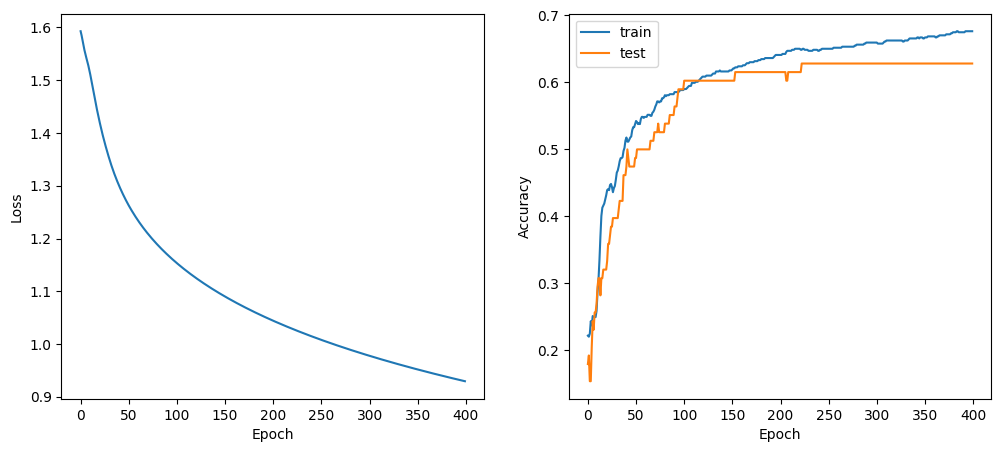
We observe that the accuracy on the test data is peaking at just over 60% accuracy. Not bad but let’s try a new model.
Second Model - 1d CNN
The second model uses a 1-Dimensional Convolutional Neural Network.
Here are two great videos to help explain the general approach and why the architecture works.
Also check this out too.
The training data for Flux CNNs must be in WHCN order; i.e. Width, Height, Channels and Number of items in the mini-batch.
size(X_train)
(200, 649)
Presently the size of X_train is 200x649. We now pick a batch size and split data into mini-batches.
using Base.Iterators: repeated, partition
batch_size = 32
mb_idxs = partition(1:size(X_train,2), batch_size)
train_set=[]
for i in mb_idxs
    push!(train_set, (X_train[:,i], y_train[:,i]))
end
The training set train_set now consists of 21 mini-batches. Each batch has 32 training (x,y) tuples with the exception of the last batch which has 9.
Now we build the 1d convolution model in Flux.
m = Chain(x -> embedding_matrix * Flux.onehotbatch(reshape(x, doc_pad_size*size(x,2)), 0:vocab_size-1),
          x -> reshape(x, max_features, doc_pad_size, 1, trunc(Int64(size(x,2)/doc_pad_size))),
          Conv((300,1), 1=>400, relu),
          x -> maxpool(x, (1,300)),
          x -> reshape(x, :, size(x,4)),
          Dense(400, 600, relu),
          Dense(600, 5),
          softmax
)
Chain(getfield(Main, Symbol("##13#17"))(), getfield(Main, Symbol("##14#18"))(), Conv((300, 1), 1=>400, NNlib.relu), getfield(Main, Symbol("##15#19"))(), getfield(Main, Symbol("##16#20"))(), Dense(400, 600, NNlib.relu), Dense(600, 5), NNlib.softmax)
Layer 1 and 2 handles the word embeddings as per model 1. The output shape from layer 2 (for the first batch) is 300×200×1x32.
Layer 3 Applies the 1d convolution filters. We use 400 channels to find new feature relationships. Activation is relu. The output size is 1x200x400x32.
Layer 4 Applies max pooling using a window size of 300x1. The output size is 1x1x400x32.
Layer 5 Flattens the shape to 400x32. This is now suitable for training in the next layer.
Layer 6 & 7 Dense layers with relu activation. Output after layer 7 will be 5x32.
Layer 7 Softmax to output probabilities per artist between 0 and 1
Whilst tuning the model I found it really useful to test the model layers on the first batch with the following command for layer 1: m[1](train_set[1][1]) and m[1:2](train_set[1][1]) for layers 1 to 2 and so on. To check the entire model is running obviously use the syntax below.
m(train_set[1][1])
Tracked 5×32 Array{Float32,2}:
 0.64655      0.0773002   0.00207123  0.643971    …  0.000502719  0.0176868
 0.121        0.891177    0.0061145   0.0336226      0.000556032  0.196564
 0.0158486    0.0108271   0.96432     0.00717857     0.000501922  0.764975
 0.216433     0.0196466   0.0274192   0.279381       0.998012     0.0190336
 0.000169021  0.00104961  7.55584e-5  0.0358473      0.000427233  0.00174087
loss_h=[]
accuracy_train=[]
accuracy_test=[]
best_acc=0.0
last_improvement=0
stat=""
accuracy(x, y) = mean(Flux.onecold(x) .== Flux.onecold(y))
loss(x, y) = sum(Flux.crossentropy(m(x), y))
optimizer = Flux.Momentum(0.004)
Momentum(0.004, 0.9, IdDict{Any,Any}())
Lets begin training the second model. Note this training loop has been modified to allow for automatic learning rate drops if the accuracy does not improve.
for epoch in 1:40
    Flux.train!(loss, Flux.params(m), train_set, optimizer)
    l = loss(X_train, y_train).data
    push!(loss_h, l)
    accuracy_trn = accuracy(m(X_train).data, y_train)
    accuracy_tst = accuracy(m(X_test).data, y_test)

    if accuracy_tst >= best_acc
        stat=" - improvement, saving model"
        BSON.@save "artist_conv.bson" m epoch accuracy_tst
        best_acc = accuracy_tst
        last_improvement=epoch
    else
        stat=" - decline"
    end

    if epoch - last_improvement >= 5
        optimizer.eta /= 10.0
        stat=" - no improvements for a while, dropping learning rate by factor of 10"
        last_improvement = epoch
    end

    if epoch - last_improvement >= 15
        stat=" - No improvement for 15 epochs STOPPING"
        break
    end

    push!(accuracy_train, accuracy_trn)
    push!(accuracy_test, accuracy_tst)
    println("$epoch -> loss= $l accuracy train=$accuracy_trn accuracy test=$accuracy_tst $stat")
end
1 -> loss= 1.5475174 accuracy train=0.4391371340523883 accuracy test=0.3333333333333333  - improvement, saving model
2 -> loss= 1.3981959 accuracy train=0.5177195685670262 accuracy test=0.4230769230769231  - improvement, saving model
3 -> loss= 1.2068622 accuracy train=0.576271186440678 accuracy test=0.46153846153846156  - improvement, saving model
4 -> loss= 1.014195 accuracy train=0.674884437596302 accuracy test=0.5256410256410257  - improvement, saving model
5 -> loss= 0.8740304 accuracy train=0.6964560862865947 accuracy test=0.5769230769230769  - improvement, saving model
6 -> loss= 0.7762191 accuracy train=0.7134052388289677 accuracy test=0.5641025641025641  - decline
7 -> loss= 0.70594215 accuracy train=0.7195685670261941 accuracy test=0.6153846153846154  - improvement, saving model
8 -> loss= 0.63908446 accuracy train=0.7411402157164869 accuracy test=0.6153846153846154  - improvement, saving model
9 -> loss= 0.5899226 accuracy train=0.7704160246533128 accuracy test=0.6025641025641025  - decline
10 -> loss= 0.5465148 accuracy train=0.7935285053929122 accuracy test=0.6025641025641025  - decline
11 -> loss= 0.58453256 accuracy train=0.7796610169491526 accuracy test=0.5769230769230769  - decline
12 -> loss= 1.08682 accuracy train=0.6332819722650231 accuracy test=0.5641025641025641  - decline
13 -> loss= 0.84157795 accuracy train=0.687211093990755 accuracy test=0.5897435897435898  - no improvements for a while, dropping learning rate by factor of 10
14 -> loss= 1.0953864 accuracy train=0.6409861325115562 accuracy test=0.5256410256410257  - decline
15 -> loss= 0.38960773 accuracy train=0.9029275808936826 accuracy test=0.6153846153846154  - improvement, saving model
16 -> loss= 0.3409845 accuracy train=0.9229583975346687 accuracy test=0.6282051282051282  - improvement, saving model
17 -> loss= 0.3086353 accuracy train=0.9291217257318952 accuracy test=0.6666666666666666  - improvement, saving model
18 -> loss= 0.2871488 accuracy train=0.938366718027735 accuracy test=0.6410256410256411  - decline
19 -> loss= 0.27186963 accuracy train=0.9414483821263482 accuracy test=0.6410256410256411  - decline
20 -> loss= 0.25938293 accuracy train=0.9460708782742681 accuracy test=0.6410256410256411  - decline
21 -> loss= 0.24849279 accuracy train=0.9460708782742681 accuracy test=0.6410256410256411  - decline
22 -> loss= 0.23899835 accuracy train=0.9491525423728814 accuracy test=0.6538461538461539  - no improvements for a while, dropping learning rate by factor of 10
23 -> loss= 0.23771816 accuracy train=0.9506933744221879 accuracy test=0.6666666666666666  - improvement, saving model
24 -> loss= 0.23479633 accuracy train=0.9522342064714946 accuracy test=0.6538461538461539  - decline
25 -> loss= 0.2335223 accuracy train=0.9522342064714946 accuracy test=0.6538461538461539  - decline
26 -> loss= 0.2326564 accuracy train=0.9506933744221879 accuracy test=0.6538461538461539  - decline
27 -> loss= 0.23182735 accuracy train=0.9491525423728814 accuracy test=0.6538461538461539  - decline
28 -> loss= 0.23101975 accuracy train=0.9491525423728814 accuracy test=0.6538461538461539  - no improvements for a while, dropping learning rate by factor of 10
29 -> loss= 0.23071226 accuracy train=0.9522342064714946 accuracy test=0.6538461538461539  - decline
30 -> loss= 0.23060969 accuracy train=0.9537750385208013 accuracy test=0.6538461538461539  - decline
31 -> loss= 0.23052704 accuracy train=0.9522342064714946 accuracy test=0.6538461538461539  - decline
32 -> loss= 0.23044708 accuracy train=0.9537750385208013 accuracy test=0.6538461538461539  - decline
33 -> loss= 0.2303679 accuracy train=0.9537750385208013 accuracy test=0.6538461538461539  - no improvements for a while, dropping learning rate by factor of 10
34 -> loss= 0.2303387 accuracy train=0.9537750385208013 accuracy test=0.6538461538461539  - decline
35 -> loss= 0.23032849 accuracy train=0.9537750385208013 accuracy test=0.6538461538461539  - decline
36 -> loss= 0.23032042 accuracy train=0.9537750385208013 accuracy test=0.6538461538461539  - decline
37 -> loss= 0.23031256 accuracy train=0.9537750385208013 accuracy test=0.6538461538461539  - decline
38 -> loss= 0.23030475 accuracy train=0.9537750385208013 accuracy test=0.6538461538461539  - no improvements for a while, dropping learning rate by factor of 10
39 -> loss= 0.23030235 accuracy train=0.9537750385208013 accuracy test=0.6538461538461539  - decline
40 -> loss= 0.23030187 accuracy train=0.9537750385208013 accuracy test=0.6538461538461539  - decline
figure(figsize=(12,5))

subplot(121)
PyPlot.xlabel("Epoch")
ylabel("Loss")
plot(loss_h)

subplot(122)
PyPlot.xlabel("Epoch")
ylabel("Accuracy")
plot(accuracy_train, label="train")
plot(accuracy_test, label="test")
legend()
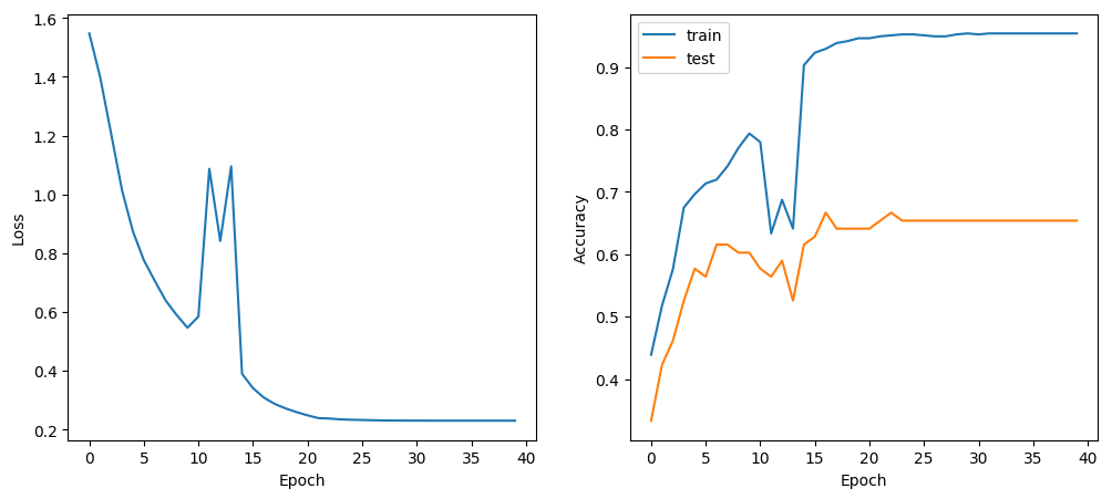
An improvement of about 4% compared to model 1.
Load the best model
You may have noticed we were saving the model as we went in the training loop if there was an accuracy improvement. The next line of code loads our best model. This step negates the need to re-run the training loop every time we run the notebook. Training can take a few minutes to run on a CPU.
The next line of code loads our trained Flux model.
BSON.@load "artist_conv.bson" m
Conclusion
The model nearly got to 70% accuracy. With a little more perseverance I think I could have got there. The steps I had in mind to improve accuracy were
-
Study and make updates to the out of vocabulary words.
-
Data augmentation and balance of training examples
I might come back to this another day….
#Function to return the artist name based on the index 'a'
function artist_name(a)
    i=findfirst(x -> x==a, artist_dict)
end
artist_name(1)
"Queen"
Put yourself to the test
Update i between 1 and 78 and put yourself to the test with the next three cells

Who wrote this song?
i=5
replace(df[649+i,:text], "\n" => " ")  # 649 is the test/train split
[Puff Intro]   Yeah   The old school   To the new school   Bad Boy, remix, let's go      [Black Rob]   Like that   Black gon'
slide with Mike Jack   Puff done remixed one hell of a track   Put me on it   I wanna know   How many want it?   Damn, it feels
good to see people love on it   For those who love slow down   'Member Motown had a brotha' happy as shit   I mean the whole
sound   Bangin' and catch six-four since we was shorties   Fee owes now rebooked from California      Carry 40's but I 'member
them times in '79   When I first started to rhyme   Sometimes I gots to look back at what it was   The good old days   The
triple o'shays when there was love      I want you back   But I can't grab that far   It's how it is   When you're living like a
star, bad boy   Come on, let's go      [Mj]   When I had you to myself   I didn't want you around   Those pretty faces   Always
made you   Stand out in a crowd   But someone picked you from the bunch   When love was all it took   Now it's much too late for
me   To take a second look      Oh baby, give me one more chance   (To show you that I love you)   Won't you please let me   (Back
in your heart)   Oh, darlin' I was blind to let you go   (Let you go baby)   But now since I see you in his arms   (I want you back)
Oh, I do now   (I want you back)   Oh, oh, baby   (I want you back)   Yeah, yeah, yeah, yeah   (I want you back)   Nah,
nah, nah, nah      Trying to live without your love   Is one long sleepless night   Let me show you girl   That I know wrong
from right   Every street you walk on   I lay tear stains on the ground   Following the girl   I didn't even want you
around      Let me tell ya now   Oh baby all I need is one more chance   (To show you that I love you)   Won't you please let
me   (Back in your heart)   Oh darlin' I was blind to let you go   (Let you go baby)   But now since I see you in his arms   (I
want you back)      [Black Rob]   It's just like Jermain Jackson   Tito, Mike and Marlon   Only think on my mind now is
stardom   Blowin' the F-up   My game's stepped up   'Member when Mike and them   First came to record   Singin' hits like
Skywriter   My Girl, People Make The World Go 'Round   Mama's Pearl, Can't Loose it   Joyful jukebox music   Never Can Say
Goodbye   That's why we use it      It's money honey   So I gots to be there   And I'm be yo Sugar Daddy   Say it's real
Versachi chair, pd, life of the party   Bad Boy, make joys for everbody      Jackson 5 Chorus in background while: [Puff Daddy]
From the old to the new   Come on   Motown   Rock on   Yeah, yeah, yeah, yeah   [Jackson 5 Chorus until fade]
Pause and think! Here is the answer.
df[649+i,[:artist, :song]]
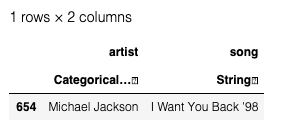
This is the prediction that model gave.
artist_name(test_predictions[i])
"Eminem"
OK so our model got it wrong, but may be you did too?
Although this one was labelled ‘Michael Jackson’ it was in the dataset as a rap remix of the his song with lyrics from P. Didy and Black Rob so I still think Eminem was the best prediction.
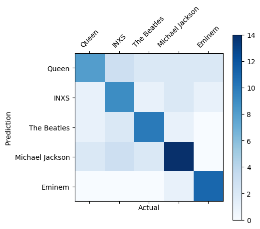
Confusion Matrix
The confusion matrix shows where the model predictions were correct (the diagonal) and where they failed (the other cells).
using MLBase
cm=confusmat(5,test_predictions, test_actual)
5×5 Array{Int64,2}:
 8  3   2   2   2
 1  9   1   2   1
 1  2  10   1   0
 2  3   2  14   0
 0  0   0   1  11
labels=[artist_name(x) for x in 1:length(artists)]
cmap=get_cmap("Blues")
cax=matshow(cm)
imshow(cm, interpolation="nearest", cmap=cmap)
colorbar()
xticks(collect(0:4), labels, rotation=45)
yticks(collect(0:4), labels)
xlabel("Actual")
ylabel("Prediction")
show()
A deeper blue means more certainty.
All Predictions
test_predictions=Flux.onecold(m(X_test))
test_actual=Flux.onecold(y_test)
showall(DataFrame(Actual = artist_name.(test_actual); Prediction = artist_name.(test_predictions)))
78×2 DataFrame
│ Row │ Actual │ Prediction │
│ │ [90mString[39m │ [90mString[39m │
├─────┼─────────────────┼─────────────────┤
│ 1 │ Queen │ Queen │
│ 2 │ Eminem │ INXS │
│ 3 │ Michael Jackson │ Michael Jackson │
│ 4 │ The Beatles │ The Beatles │
│ 5 │ Michael Jackson │ Eminem │
│ 6 │ INXS │ INXS │
│ 7 │ Eminem │ Eminem │
│ 8 │ Eminem │ Eminem │
│ 9 │ Eminem │ Queen │
│ 10 │ The Beatles │ The Beatles │
│ 11 │ The Beatles │ The Beatles │
│ 12 │ The Beatles │ Michael Jackson │
│ 13 │ INXS │ Queen │
│ 14 │ The Beatles │ The Beatles │
│ 15 │ Michael Jackson │ Michael Jackson │
│ 16 │ Queen │ Queen │
│ 17 │ Michael Jackson │ Michael Jackson │
│ 18 │ INXS │ INXS │
│ 19 │ Michael Jackson │ Michael Jackson │
│ 20 │ Michael Jackson │ Michael Jackson │
│ 21 │ Michael Jackson │ Michael Jackson │
│ 22 │ Eminem │ Eminem │
│ 23 │ INXS │ INXS │
│ 24 │ INXS │ INXS │
│ 25 │ Queen │ Queen │
│ 26 │ Michael Jackson │ Michael Jackson │
│ 27 │ The Beatles │ Queen │
│ 28 │ Eminem │ Eminem │
│ 29 │ INXS │ Michael Jackson │
│ 30 │ The Beatles │ Michael Jackson │
│ 31 │ Michael Jackson │ The Beatles │
│ 32 │ Queen │ Queen │
│ 33 │ Michael Jackson │ Michael Jackson │
│ 34 │ Michael Jackson │ INXS │
│ 35 │ INXS │ Queen │
│ 36 │ Michael Jackson │ Michael Jackson │
│ 37 │ Queen │ Queen │
│ 38 │ INXS │ Michael Jackson │
│ 39 │ INXS │ INXS │
│ 40 │ Eminem │ Queen │
│ 41 │ The Beatles │ The Beatles │
│ 42 │ INXS │ INXS │
│ 43 │ The Beatles │ The Beatles │
│ 44 │ Michael Jackson │ Michael Jackson │
│ 45 │ Michael Jackson │ Michael Jackson │
│ 46 │ INXS │ Michael Jackson │
│ 47 │ The Beatles │ The Beatles │
│ 48 │ INXS │ The Beatles │
│ 49 │ Eminem │ Eminem │
│ 50 │ Eminem │ Eminem │
│ 51 │ Michael Jackson │ Michael Jackson │
│ 52 │ INXS │ The Beatles │
│ 53 │ The Beatles │ The Beatles │
│ 54 │ Eminem │ Eminem │
│ 55 │ Queen │ Michael Jackson │
│ 56 │ Michael Jackson │ INXS │
│ 57 │ Queen │ Queen │
│ 58 │ Eminem │ Eminem │
│ 59 │ Eminem │ Eminem │
│ 60 │ Queen │ Michael Jackson │
│ 61 │ INXS │ INXS │
│ 62 │ INXS │ Queen │
│ 63 │ INXS │ INXS │
│ 64 │ Queen │ Queen │
│ 65 │ Michael Jackson │ Michael Jackson │
│ 66 │ Queen │ INXS │
│ 67 │ Eminem │ Eminem │
│ 68 │ Eminem │ Eminem │
│ 69 │ Queen │ The Beatles │
│ 70 │ Queen │ Queen │
│ 71 │ The Beatles │ The Beatles │
│ 72 │ The Beatles │ Queen │
│ 73 │ The Beatles │ The Beatles │
│ 74 │ Michael Jackson │ Michael Jackson │
│ 75 │ The Beatles │ INXS │
│ 76 │ Michael Jackson │ Queen │
│ 77 │ Michael Jackson │ Queen │
│ 78 │ INXS │ INXS │
Let me know if anything could be improved.
Leave a comment