Julia Flux Simple Regression Model

Flux is a Neural Network Machine Learning library for the Julia programming language. Flux may be likened to TensorFlow but it shows potential to be easier as there is no additional ‘graphing’ language layer to learn – it’s just plain Julia.

Let’s get started with a simple example.

using Distributions, PyPlot, Random, Flux

#Display Flux Version
import Pkg ; Pkg.installed()["Flux"]

v"0.7.2"

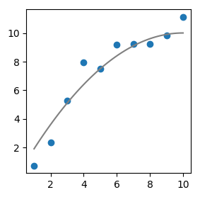
Generate some data randomly distributed about the polynomial function \(-0.1x^2 + 2x\)

f(x) = -0.1*x^2 + 2*x
Random.seed!(1000)
x = collect(1:10)
y = [f(i) for i in x] .+ rand(Normal(0,0.75),10)

#Plot f(x) and models using n data points
n=100
x_rng=LinRange(1, 10, n)

figure(figsize=(3,3))
scatter(x,y)
plot(x_rng,f.(x_rng), color="gray")
show()

The Julia function below takes the inputs of our ‘random’ data \(x, y\) and returns a one of two trained Flux models. The goal is to predict a fit close to the known polynomial f(x).

Model 1 is the most trivial with one dense input; i.e. \(y = σ.(W * x .+ b)\)

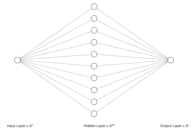
Model 2 has 1 hidden layer with a definable amount of neurons for experimentation

Training is done with the optimiser : Gradient Descent

NOTE: σ = identity = i.e. the identity matrix for regression

function train_model(x, y, hl_neurons=0)
    
    # x must be an `in` × N matrix
    x = x'
    
    # Create data iterator for 1000 epochs
    data_iterator = Iterators.repeated((x, y), 1000)
    
    # Set-up model layout
    if hl_neurons==0
        m = Chain(Dense(1,1), identity)
    else
        m = Chain(Dense(1, hl_neurons, tanh),
                  Dense(hl_neurons, 1, identity))
    end
    
    #Our loss function to minimize
    loss(x, y) = sum((m(x) .- y').^2)
    optimizer = Flux.Descent(0.0001)
    Flux.train!(loss, Flux.params(m), data_iterator, optimizer)
    return m
end

Make predictions and plot against our source data. Note, in the example I included 10 neurons.

model=train_model(x, y)
y_linear=reshape(model(x').data, length(x),)

model=train_model(x, y, 10)
y_hid=reshape(model(x_rng').data, n,)

figure(figsize=(12,5))

subplot(121)
scatter(x,y)
plot(x_rng,f.(x_rng), color="gray", label="Source Polynomial f(x)")
plot(x,y_linear, label="Predictions using Dense Layer Model")
legend()

subplot(122)
scatter(x,y)
plot(x_rng,f.(x_rng), color="gray", label="Source Polynomial f(x)")
plot(x_rng,y_hid, label="Predictions using Hidden Layer Model")
legend()
show()

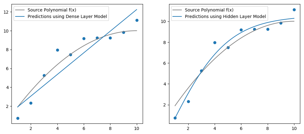
The introduction of the hidden layer approximates our function well! Apparently, a one layer neural network can approximate any continuous function. I might put this to the test another day.

The trained parameters of the model can be obtained with Flux.params(model). For the 10-neuron model you end up with 10 sets of parameters for the trained weights and biases. You cannot approximate the original polynomial co-efficients of f(x) as such.