Julia Word Embedding Layer in Flux - Self Trained

In this example we take a look at how to use an embedding layer in Julia with Flux. If you need help on what embeddings are check out this page and then return here to see how we can use them as the first layer in a neural network.

The objective for this exercise is to machine learn the sentiment of 10 string arrays. The idea came from this tutorial written by Jason Brownlee who used Keras on a similar dataset.

using  Languages, TextAnalysis, Flux, PyPlot, Statistics

#Display Flux Version
import Pkg ; Pkg.installed()["Flux"]

v"0.7.2"

Data Preparation

The first block of code defines our training ‘documents’ and labels (y).

Arr = ["well done",
     "good work",
     "great effort",
     "nice work",
     "excellent",
     "weak",
     "poor effort",
     "not good",
     "poor work",
     "could have done better"]

# positve or negative sentiment to each 'document' string
y = [true true true true true false false false false false]

Next we set up a dictionary of words used. Each word points to an integer index. To do this the TextAnalysis package was used. If you’re interested in how this works watch this video.

docs=[]
for i in 1:length(Arr)
    push!(docs, StringDocument(Arr[i]))
end
crps=Corpus(docs)    
update_lexicon!(crps)
doc_term_matrix=DocumentTermMatrix(crps)
word_dict=doc_term_matrix.column_indices

Dict{String,Int64} with 14 entries:
  "done"      => 3
  "not"       => 10
  "excellent" => 5
  "have"      => 8
  "well"      => 13
  "work"      => 14
  "nice"      => 9
  "effort"    => 4
  "great"     => 7
  "poor"      => 11
  "could"     => 2
  "better"    => 1
  "good"      => 6
  "weak"      => 12

The following function returns the index of the word in the word dictionary and returns 0 if the word is not found.

tk_idx(s) = haskey(word_dict, s) ? i=word_dict[s] : i=0

The following function is used to ensure each document in the corpus has an equal length.

function pad_corpus(c, pad_size)
    M=[]
    for doc in 1:length(c)
        tks = tokens(c[doc])
        if length(tks)>=pad_size
            tk_indexes=[tk_idx(w) for w in tks[1:pad_size]]
        end
        if length(tks)<pad_size
            tk_indexes=zeros(Int64,pad_size-length(tks))
            tk_indexes=vcat(tk_indexes, [tk_idx(w) for w in tks])
        end
        doc==1 ? M=tk_indexes' : M=vcat(M, tk_indexes')
    end
    return M
end

The final step in our data preparation creates a dense matrix where the numbers greater than zero relate to a word. As the maximum document length is 4 (i.e. “could have done better”) we will use the pad size of 4. The matrix is transposed ready for training whereby each column represents one document.

pad_size=4
padded_docs = pad_corpus(crps, pad_size)
x = padded_docs'
data = [(x, y)]

x

  0   0  0   0  0   0   0   0   0  2
  0   0  0   0  0   0   0   0   0  8
 13   6  7   9  0   0  11  10  11  3
  3  14  4  14  5  12   4   6  14  1

Flux Embedding Preparation

Next let’s get ready for the embedding layer. In this example we’ll learn 8 features per word but for a larger corpus you’ll probably need a higher dimension, perhaps even 300. The vocab size is set to 20 which is higher than the maximum index in our dictionary.

N = size(padded_docs,1)  #Number of documents (10)
max_features = 8
vocab_size = 20

The next block of code sets up a Julia constructor called EmbeddingLayer. The layer is initialized with a special random initializer called glorot_normal. Also note Flux must be set to treelike otherwise it will not update/learn the embeddings.

struct EmbeddingLayer
   W
   EmbeddingLayer(mf, vs) = new(param(Flux.glorot_normal(mf, vs)))
end

@Flux.treelike EmbeddingLayer

(m::EmbeddingLayer)(x) = m.W * Flux.onehotbatch(reshape(x, pad_size*N), 0:vocab_size-1)

Buliding the Model and Training

The model needs some explanation.

Layer 1. As x is fed into the model, the first layer’s embedding function matches the words in each document to corresponding word vectors. This is done by rolling all the word vectors one after the other and using onehotbatch to filter out the unwanted words. The output is a 8x40 array.

Layer 2. Unrolls the vectors into the shape 8x4x10; i.e. 8 features and 10 documents of padded size 4.

Layer 3. Now that our data is in the shape provided by layer 2 we can sum the word vectors to get an overall ‘meaning’ vector for each document. The output is now in the shape size of 8 x 1 x 10.

Layer 4: Drops an axis so that the shape of x is a size suitable for training. After this step the shape is 8x10.

Layer 5: is a normal Dense layer with the sigmoid activation function to give us nice probabilities.

If you’d like to see each layer in action I recommend using m[1](x) to see sample output from the first layer. m[1:2](x) to see output from the second layer and so on.

m = Chain(EmbeddingLayer(max_features, vocab_size),
          x -> reshape(x, max_features, pad_size, N),
          x -> sum(x, dims=2),
          x -> reshape(x, max_features, N),
          Dense(max_features, 1, σ)
)

Chain(EmbeddingLayer(Float32[0.278128 0.111989 … -0.244614 -0.377189; 0.0647178 0.0683725 … -0.112626 -0.434706; … ; 0.397401 0.407925 … 0.438091 0.0588613; -0.361919 -0.114776 … -0.356307 -0.10119] (tracked)), getfield(Main, Symbol("##3#6"))(), getfield(Main, Symbol("##4#7"))(), getfield(Main, Symbol("##5#8"))(), Dense(8, 1, NNlib.σ))

Now let’s initialize some arrays and create a function to calculate accuracy.

loss_h=[]
accuracy_train=[]
accuracy(x, y) = mean(x .== y)

As this is a binary (1 or 0) classification problem we need to use binarycrossentropy to calculate the loss. The optimizer is gradient descent.

loss(x, y) = sum(Flux.binarycrossentropy.(m(x), y))
optimizer = Flux.Descent(0.01)

Train the model.

for epoch in 1:400
    Flux.train!(loss, Flux.params(m), data, optimizer)
    #println(loss(x, y).data, " ", accuracy(m(x).>0.5,y))
    push!(loss_h, loss(x, y).data)
    push!(accuracy_train, accuracy(m(x).>0.5,y))
end
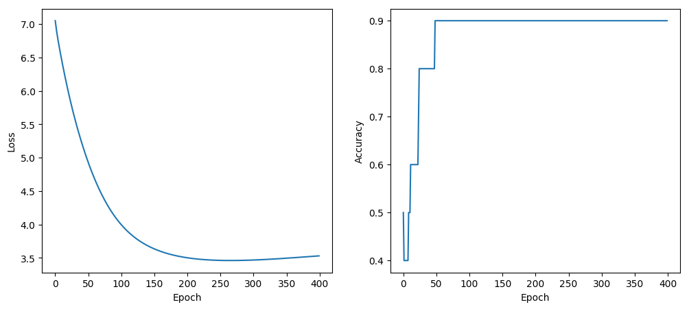
println(m(x).>0.5)
accuracy(m(x).>0.5,y)

Bool[true false true true true false false false false false]
0.9

Outputs over 0.5 are considered positive (true) and our final accuracy is 90%.

The second example is incorrectly scored as false. I think this is because the words “good” and “work” also appear in the negative examples. Next we’ll see what happens using the pre-trained word embeddings.

figure(figsize=(12,5))

subplot(121)
PyPlot.xlabel("Epoch")
ylabel("Loss")
plot(loss_h)

subplot(122)
PyPlot.xlabel("Epoch")
ylabel("Accuracy")
plot(accuracy_train, label="train")

Note, some parts of this could be done more elegantly, let me know.